Introduction

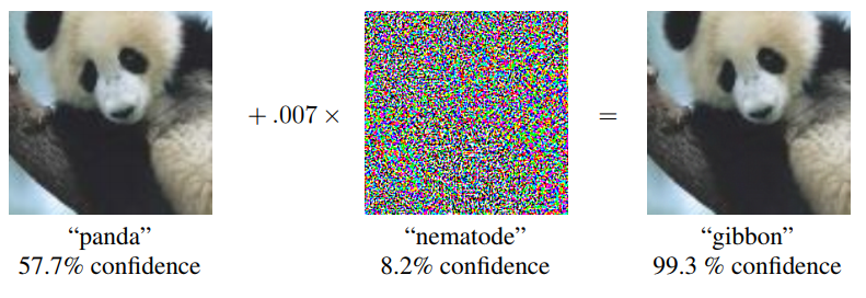
A lot of academic attention has been focused on the topic of adversarial attacks against neural networks recently, and for good reason. Because we still lack a thorough understanding of why neural networks work well, the failure modes of neural networks are quite surprising¹. By injective noise which is imperceptible to human vision, it is possible to fool a network into misclassifying an input image with very high confidence. The classic attack called the Fast Gradient Sign Method (FGSM) is shown below and can be implemented in just a few lines of code.

There are already plenty of resources explaining the basics of neural networks and backpropagation, so I’ll just quickly summarize the basics here. The standard formulation of training a neural network is that of minimizing a loss function defined with respect to the weights/parameters of the neural network. In practice this is usually an empirical loss function, i.e. the loss of the network’s predictions averaged over a finite and fixed dataset:

\[\arg \min_{\theta} \frac{1}{N}\sum_{i=1}^N{l(x_i, y_i; \theta)}\]

for $\theta$ the parameters of the network, $l(\theta;x, y)$ the loss function defined on the parameters of the network with respect to a training input $x$ and label $y$.

The gold standard of optimization algorithms remains Stochastic Gradient Descent (SGD), where we iteratively update the parameters of the network in the opposite direction of the gradient with respect to the parameters. Because we choose the architecture of a neural network and its loss function to be differentiable, it is also possible to differentiate the loss function with respect to the input $x_i$.

In order to attack a neural network, we can just flip the original optimization objective on its head. In an untargeted attack, we wish to reduce overall accuracy of the network and can simply maximize the same loss function. In a targeted attack, we wish to convince the network that an input image belongs to an arbitrary class of our choosing. We also add a constraint bounding the maximum norm of the perturbation and our optimization problem in a simple untargeted attack becomes:

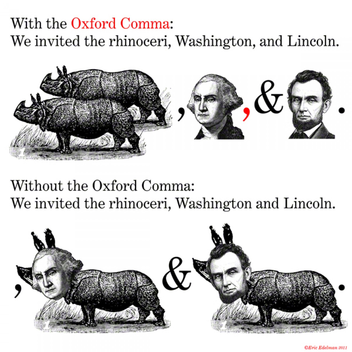
\[\arg \max \quad l(x + \delta, y; \theta)\\ \text{subject to} \quad \|\delta\|_p < \epsilon\]

A key assumption of many adversarial attacks is that a small perturbation does not affect the semantic content of the input, which generally holds in the domain of natural images. In the domain of natural language, however, it has been well documented by comedians on the internet that changing a single word or even punctuation mark can drastically alter the meaning of a sentence.

There are a wide variety of algorithms which have been designed specifically for this inverted optimization problem which work quite well. In both of these scenarios, we assume full knowledge of both the architecture and the weights of the neural network. These are known as “whitebox” attacks as opposed to “blackbox” attacks. Due to the transfer learning properties of neural networks, however, it is possible to create adversarial attacks even without knowledge of architecture and weights by training a similar architecture on a similar dataset. Surprisingly, whitebox attacks on this voodoo doll network transfer well to the original blackbox target.

Methods

In any case, most of these results published previously deal with the case of attacking a fixed input. As the adversarial perturbations are only computed with respect to a particular input, they lose their efficacy when applied to other inputs or slightly transformed. Is it at all possible, then, to create adversarial perturbations that work across a variety of transformations? It turns out that the naive approach of just optimizing the average adversarial objective function across all transformations works quite well. Our untargeted attack from above becomes:

\[\arg \max \quad \mathbb{E}_{t \sim T, x \sim X} [l(x + \delta, y; \theta)]\\ \text{subject to} \quad \mathbb{E}_{t \sim T, x \sim X} [\|\delta\|_p < \epsilon]\]

for $T$ the distribution of transformations and $X$ the distribution of inputs. In practice the expectation is replaced by a sample mean over a random sample of transformations and inputs.

This is the main insight behind the paper Adversarial Patch which uses the above optimization framework to train a single adversarial patch which can fool a classifier with high probability when applied on top of arbitrary images, under arbitrary transformations. Given a patch $p$ of some fixed size and an image $x$, they define a patch application operator $A(p, x, t)$ which applies the patch to $x$ after rotating, scaling, and translating by transformation parameter $t$. If we implement the rotation, scaling, and translation through a single affine transformation, the entire operator $A$ is differentiable with respect to the patch $p$.

Replacing the generic loss function above with the log probability of our target class as well as the noise application with our patch application, we arrive at out final optimization objective which we also optimize with SGD:

\[\arg \max_{p} \quad \mathbb{E}_{t \sim T, x \sim X} [\log \text{Pr}(\hat{y} | A(p, x, t); \theta))]\]

Results

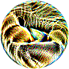
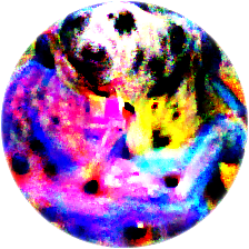
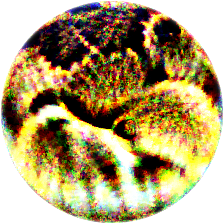
I re-implemented the Adversarial Patch code in PyTorch and after 500 SGD iterations at a minibatch size of 16, with transformation angle in degrees sampled from [-22.5, 22.5], scale factor sampled from [0.1, 0.9], and location sampled uniformly at random from all locations where the entire patch remains in the image frame, i.e. no part is clipped. With the target class set to toaster, running the attack on a pretrained ResNet50 neural network gives us the following patch:

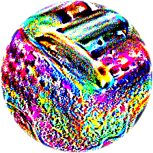
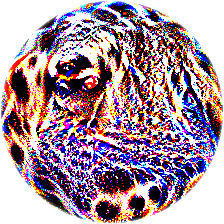
Our patch looks somewhat like a toaster, though perhaps this is just a coincidence. Repeating the attack with target classes of dalmation and rattlesnake, we confirm that each patch does indeed bear an abstract resemblance to its target class. In the original paper, the authors conjecture that the adversarial patch attack works by essentially computing a very high saliency version of the underlying target class which drowns out the original class in the image, and our results here are consistent with this hypothesis.

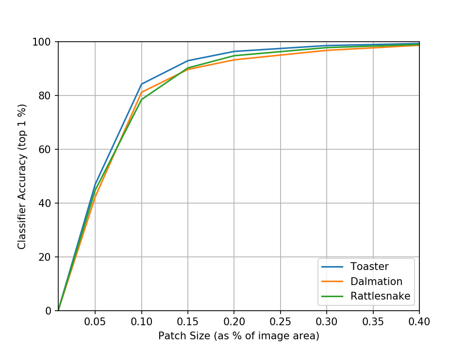
We can also measure the attack success rate against the size of the patch²:

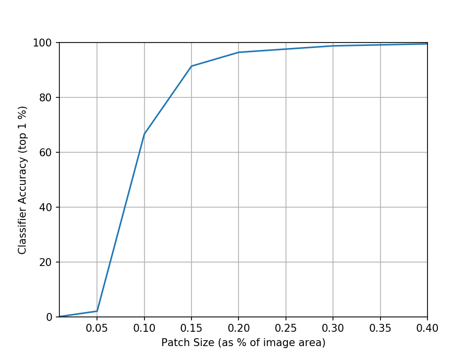
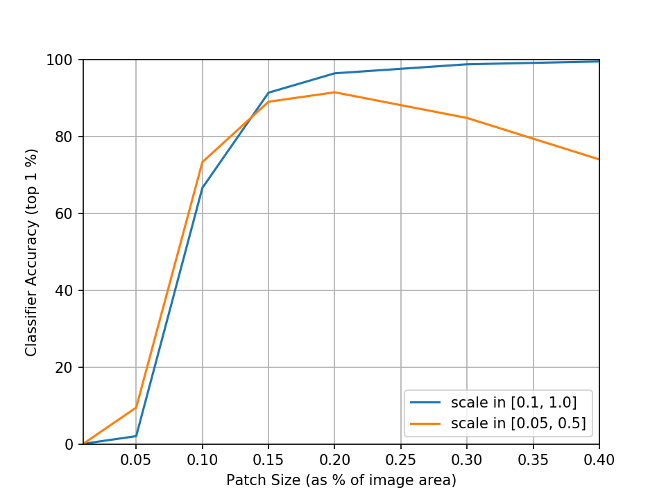
Quite intuitively, we can see that as we reduce the size of the patch it becomes more and more difficult to pull off a successful attack. We can somewhat mitigate this by shifting the range of sampled scale factors down to focus more on smaller scales which also are more realistic. Sampling the scale instead from the range 0.05 to 0.5 (which corresponds to 2% to 20% of the image area) indeed gives us improved performance at smaller sizes but interestingly also loses some performance at higher sizes which don’t appear during training.

At this point I decided to experiment with adding a regularization term which penalizes large distances between neighboring pixels of the patch to see if it would give us less noisy patches. I decided to use a variant of total variation:

\[v_{\text{aniso}}(y) = \sum_{i, j}\|y_{i+1, j} - y_{i,j}\| + \|y_{i, j+1} - y_{i,j}\|\]

Since the sum of distances between all pairs of neighboring pixels ends up being quite large, I then scaled the total variation term down by 0.0001 before adding it to the previous loss. Re-running the original baseline with this new total variation term gives us the following patch:

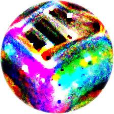
The total variation regularized patch is much smoother and more strongly resembles a real toaster. Total variation regularized patches with target classes of dalmation and rattlesnake also realistically resemble their respective classes:

We also see a dramatic increase in attack success rate at 5% of image area from 2% to 46% and at 10% of image area from 67% to 84%. I suspect this is because the total variation regularized patch avoids the noisy structure present in the baseline patch which gets destroyed when scaling down to 5-10% and thus fares better at those sizes.

To me, the most surprising part of these results is how effective the adversarial patch works. With a batch size of 16 and trained with 500 iterations, each patch is trained on just 8000 images. Yet at just 5% of the image area, the patch is successful at fooling the classifier over 40% of the time! I ran some additional experiments which train for more iterations and anneal the learning rate and found further, albeit minor improvements. You can find the code used in these experiments at http://github.com/normster/adversarial_patch_pytorch.